Sur crash course
This is a tutorial to dive in the key concepts of Sur and its usage under an interactive session.
Getting up
Sur has an object-oriented design. This means that the library provides classes to interact with. The very first step is to import the classes and some helper functions we will need.
In [1]:
from sur import Mixture, Compound, EosSetup, EosEnvelope, EosFlash, ExperimentalEnvelope, setup_database
We also need to create the database and load the built-in dataset of pure components constants. By default, Sur uses a database in memory, which is not persistence.
In [2]:
setup_database()
We are ready to start.
Define a mixture
As you know, a mixture is two or more compound which have been combined
such that each substance retains its own chemical identity. A
Mixture in sur is the same: a combination of compounds, each one
with its fraction (i.e, the sum of the fractions of all the compounds in
the mixture must be 1)
In [3]:
mixture = Mixture()
There are several ways to add compounds to a Mixture instance. For
instance, you can use as if it would be a dictionary.
In [4]:
mixture["co2"] = 0.5
mixture["n-decane"] = 0.25
mixture["methane"] = 0.25
In order to facilitate the definition of interaction matrixes, we could sort each fraction by its molecular weight, no matter the order we added them.
In [5]:
mixture.sort()
In [6]:
mixture
Out[6]:
[(<Compound: METHANE>, Decimal('0.25')), (<Compound: CARBON DIOXIDE>, Decimal('0.5')), (<Compound: n-DECANE>, Decimal('0.25'))]
Setup the EoS
To simulate the envelope, we need to choice and configurate an Equation
of State. This is done via an EosSetup instance. For example, to use
an RK-PR EoS with parameters \(k_{ij}\) and \(l_{ij}\) as
constants, we create a setup object like this:
In [7]:
setup = EosSetup.objects.create(eos='RKPR', kij_mode=EosSetup.CONSTANTS, lij_mode=EosSetup.CONSTANTS)
By default, the interaction parameter between two compounds is 0.0 (however, Sur may provide a better choice when appropiated). To customize the calculation with our own parameters, we can override the default values.
In [8]:
setup.set_interaction('kij', 'methane', 'co2', 0.1)
setup.set_interaction('kij', 'co2', 'n-decane',  0.091)
Out[8]:
<KijInteractionParameter: RKPR [<Compound: CARBON DIOXIDE>, <Compound: n-DECANE>]: 0.091>
A setup object is independent of a mixture. It just define the equation to be used and the bag of parameters to tune it when we simulate an envelope for a particular mixture, but to have interaction between compounds that don’t belong to a mixture is perfectly valid.
After set the interaction parameter, we probably want to see how the interaction matrix looks like for our particular compounds
In [9]:
setup.kij(mixture)
Out[9]:
array([[ 0.   ,  0.1  ,  0.   ],
       [ 0.1  ,  0.   ,  0.091],
       [ 0.   ,  0.091,  0.   ]])
By the way, it’d be also possible to define the whole matrix for a
particular mixture at once, using the method
setup.set_interaction_matrix()
Simulate the envelope
Having the mixture and the setup, we are able to obtain a the simulated envelope.
In [10]:
envelope = mixture.get_envelope(setup)
In this case, envelope is an instance of EosEnvelope, i.e. an
envelope that have been created via an equation of state.
Any kind of envelope has many attributes ready to be inspected. For instance, we have the array of pressure and temperature
In [11]:
envelope.p
Out[11]:
array([  1.44200000e-02,   1.64600000e-02,   2.01600000e-02,
         2.45700000e-02,   2.97800000e-02,   3.59200000e-02,
         4.31100000e-02,   5.14700000e-02,   6.11500000e-02,
         7.22700000e-02,   8.49900000e-02,   9.94400000e-02,
         1.15800000e-01,   1.34100000e-01,   1.54500000e-01,
         1.77100000e-01,   2.02000000e-01,   2.29200000e-01,
         2.58800000e-01,   2.90700000e-01,   3.24900000e-01,
         4.05600000e-01,   5.23400000e-01,   6.71100000e-01,
         8.54900000e-01,   1.08200000e+00,   1.36100000e+00,
         1.70100000e+00,   2.11100000e+00,   2.60400000e+00,
         3.19200000e+00,   3.88700000e+00,   4.70400000e+00,
         5.65700000e+00,   6.75900000e+00,   8.02800000e+00,
         9.47500000e+00,   1.11200000e+01,   1.29700000e+01,
         1.50400000e+01,   1.73400000e+01,   1.98900000e+01,
         2.26900000e+01,   2.57500000e+01,   2.90700000e+01,
         3.26600000e+01,   3.65200000e+01,   4.06600000e+01,
         4.50600000e+01,   4.97300000e+01,   5.46600000e+01,
         5.98400000e+01,   6.52700000e+01,   7.09400000e+01,
         7.71600000e+01,   8.40100000e+01,   9.15900000e+01,
         1.00000000e+02,   1.09400000e+02,   1.18800000e+02,
         1.27600000e+02,   1.35800000e+02,   1.43600000e+02,
         1.50900000e+02,   1.54400000e+02,   1.64100000e+02,
         1.70000000e+02,   1.75400000e+02,   1.80400000e+02,
         1.84800000e+02,   1.88700000e+02,   1.92100000e+02,
         1.95000000e+02,   1.97400000e+02,   1.99300000e+02,
         2.00700000e+02,   2.01200000e+02,   2.01600000e+02,
         2.01800000e+02,   2.02000000e+02,   2.02000000e+02,
         2.01600000e+02,   2.01200000e+02,   2.00700000e+02,
         2.00000000e+02,   1.99200000e+02,   1.98200000e+02,
         1.97100000e+02,   1.95900000e+02,   1.94600000e+02,
         1.93300000e+02,   1.90200000e+02,   1.88200000e+02,
         1.86100000e+02,   1.83900000e+02,   1.81700000e+02,
         1.79400000e+02,   1.74600000e+02,   1.72000000e+02,
         1.66500000e+02,   1.60900000e+02,   1.55200000e+02,
         1.49500000e+02,   1.43900000e+02,   1.38400000e+02,
         1.33100000e+02,   1.28000000e+02,   1.23000000e+02,
         1.18400000e+02,   1.13900000e+02,   1.09600000e+02,
         1.05500000e+02,   1.01700000e+02,   9.79600000e+01,
         9.44300000e+01,   9.10500000e+01,   8.78100000e+01,
         8.47000000e+01,   8.17100000e+01,   7.88300000e+01,
         7.60400000e+01,   7.33500000e+01,   7.07400000e+01,
         6.82100000e+01,   6.57500000e+01,   6.33700000e+01,
         6.10400000e+01,   5.87900000e+01,   5.65900000e+01,
         5.44400000e+01,   5.23600000e+01,   5.03300000e+01,
         4.83500000e+01,   4.64300000e+01,   4.45600000e+01,
         4.27400000e+01,   4.09700000e+01,   3.92500000e+01,
         3.75900000e+01,   3.59700000e+01,   3.44000000e+01,
         3.28800000e+01,   3.14100000e+01,   2.99800000e+01,
         2.86000000e+01,   2.72700000e+01,   2.59800000e+01,
         2.47400000e+01,   2.35400000e+01,   2.23900000e+01,
         2.12800000e+01,   2.02100000e+01,   1.91800000e+01,
         1.81900000e+01,   1.72400000e+01,   1.63300000e+01,
         1.54500000e+01,   1.46200000e+01,   1.38100000e+01,
         1.30500000e+01,   1.23100000e+01,   1.16100000e+01,
         1.09400000e+01,   1.03000000e+01,   9.69100000e+00,
         9.11100000e+00,   8.55800000e+00,   8.03200000e+00,
         7.53200000e+00,   7.05800000e+00,   6.60800000e+00,
         6.18100000e+00,   5.77700000e+00,   5.39400000e+00,
         5.03200000e+00])
In [12]:
envelope.t
Out[12]:
array([ 310.    ,  312.0833,  315.3334,  318.5817,  321.8256,  325.0618,
        328.287 ,  331.4979,  334.6908,  337.8618,  341.0071,  344.1223,
        347.2033,  350.2456,  353.2444,  356.1952,  359.0929,  361.9326,
        364.7092,  367.4176,  370.0526,  375.4492,  381.889 ,  388.4249,
        395.0497,  401.7551,  408.5312,  415.3667,  422.2482,  429.1612,
        436.0893,  443.0145,  449.9174,  456.7773,  463.5724,  470.2797,
        476.8758,  483.3365,  489.6373,  495.7541,  501.6625,  507.3389,
        512.7602,  517.904 ,  522.749 ,  527.2748,  531.462 ,  535.2922,
        538.7482,  541.8137,  544.4731,  546.7121,  548.5169,  549.8788,
        550.8162,  551.236 ,  551.015 ,  549.9858,  547.9151,  544.911 ,
        541.2341,  536.9976,  532.2864,  527.1669,  524.4715,  515.914 ,
        509.8688,  503.5958,  497.1301,  490.5047,  483.751 ,  476.8995,
        469.9794,  463.0191,  456.0457,  449.0857,  445.4863,  441.9006,
        438.332 ,  434.7837,  431.2588,  424.291 ,  420.3194,  416.3945,
        412.5202,  408.7   ,  404.9371,  401.2346,  397.5952,  394.0213,
        390.5151,  383.7132,  379.7462,  375.8867,  372.1359,  368.4946,
        364.9629,  358.2265,  354.6604,  347.9187,  341.4057,  335.2389,
        329.4222,  323.9512,  318.8144,  313.9956,  309.4744,  305.2285,
        301.2344,  297.4685,  293.9078,  290.5301,  287.3146,  284.2421,
        281.2947,  278.4564,  275.7124,  273.0497,  270.4565,  267.9224,
        265.4384,  262.9962,  260.589 ,  258.2107,  255.8562,  253.5209,
        251.2014,  248.8943,  246.5974,  244.3085,  242.0261,  239.7491,
        237.4765,  235.2078,  232.9426,  230.681 ,  228.423 ,  226.1689,
        223.9189,  221.6736,  219.4335,  217.1993,  214.9716,  212.7511,
        210.5385,  208.3345,  206.1399,  203.9553,  201.7815,  199.6192,
        197.4689,  195.3314,  193.2072,  191.097 ,  189.0011,  186.9202,
        184.8547,  182.8049,  180.7714,  178.7545,  176.7545,  174.7718,
        172.8065,  170.8589,  168.9294,  167.0179,  165.1248,  163.2502,
        161.3942,  159.5569,  157.7385,  155.9389,  154.1583,  152.3968,
        150.6543])
There is also equivalent arrays for critical points, if any. In our example there is just one point.
In [13]:
envelope.t_cri, envelope.p_cri
Out[13]:
(array([ 520.3626]), array([ 159.1]))
Plotting
In addition, an envelope object is able to generate a predefined Matplotlib figure. Before run it, if you are using Sur through Jupyter, may be handy to use the magic command to embed matplotlib figures directly in the document (instead of raise a popup window)
In [14]:
%matplotlib inline
In [15]:
fig = envelope.plot()
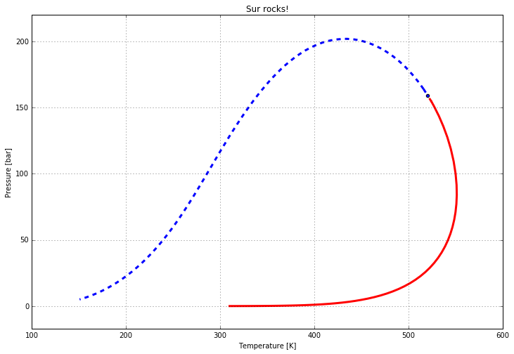
As we saved the figure object (fig), we can use the matplotlib
API to manipulate it
(changing aspect, size, span, colors..., in fact, anything we want),
export, etc.
In [16]:
from matplotlib import pyplot as plt

ax = fig.get_axes()[0]
ax.set_yticks([0] + ax.get_yticks()[1:])
ax.set_ylim((-50/3, 220))
ax.set_title('Sur rocks!')
plt.setp(ax.lines, linewidth=3)
plt.setp(ax.lines[1:], linestyle='--')
fig.set_size_inches(fig.get_size_inches() * 2)
fig
Out[16]:
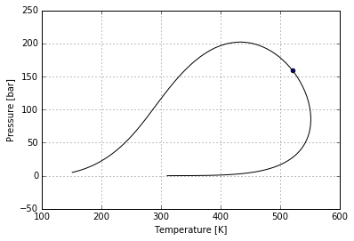
However, if that is too much power to your goal, you can pass some
format directives (as in pyplot’s
`plot() <http://matplotlib.org/users/pyplot_tutorial.html>`__)
directly to the method’s parameters. For example:
In [17]:
envelope.plot(format='k');
In [18]:
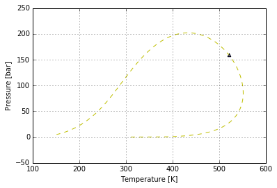
envelope.plot(critical_point='^', format='--y');
Compare with experimental data
Constrant the simulation against a known experimental dataset for an evelope is possible. Here we’ll mock this experimental data modifing the simulated one, but you should get it from a reliable source
In [19]:
import numpy as np
n = envelope.p.size

p_experimental = envelope.p[np.arange(0, n, 7)]  * 1.1
t_experimental = envelope.t[np.arange(0, n, 7)]
exp_envelope = mixture.experimental_envelope(t_experimental, p_experimental)
In this case, the exp_envelope object is an instance of
ExperimentalEnvelope. In many way it works identically than an
EosEnvelope (strictly, both are subclasses of the same base class), and
they share attribute and methods. Of course, the key difference for an
experimental envelope is that we don’t need to calculate, we just set
the arrays manually.
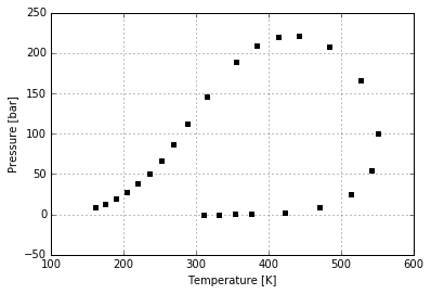
Another difference is that the default plot style is slightly different.
In [20]:
exp_fig = exp_envelope.plot()
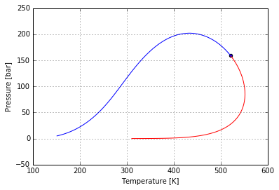
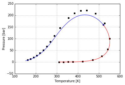
By the way, many envelope’s figures can be chained, passing a base one
to the method plot() as the first parameter. For example, here we
plot both the simulated and the experimental envelopes in the same
figure
In [21]:
envelope.plot(exp_fig)
Out[21]:
Calculate a flash
A flash represents a separation of the mixture in two with the same
compounds but different fractions. In Sur, we can get a flash instance
through the method get_flash()
In [22]:
flash = mixture.get_flash(setup, t=400, p=100)
In [23]:
flash.vapour_mixture
Out[23]:
[(<Compound: METHANE>, Decimal('0.360497')), (<Compound: CARBON DIOXIDE>, Decimal('0.625358')), (<Compound: n-DECANE>, Decimal('0.014145'))]
In [24]:
flash.liquid_mixture.z
Out[24]:
array([ 0.116292, 0.348308, 0.5354 ])
Which is the same than
In [25]:
flash.x
Out[25]:
array([ 0.116292, 0.348308, 0.5354 ])
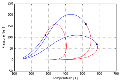
The liquid_mixture and vapour_mixture attributes are Mixture
objects, meaning we can get its own evelopes and the plot all together
In [26]:
le = flash.liquid_mixture.get_envelope(setup)
ve = flash.vapour_mixture.get_envelope(setup)

final_fig = envelope.plot(ve.plot(le.plot()))